AutoBNN: Probabilistic time series forecasting with compositional bayesian neural networks
March 28, 2024
Posted by Urs Köster, Software Engineer, Google Research
AutoBNN combines the interpretability of traditional probabilistic approaches with the scalability and flexibility of neural networks for building sophisticated time series prediction models using complex data.
Quick links
Time series problems are ubiquitous, from forecasting weather and traffic patterns to understanding economic trends. Bayesian approaches start with an assumption about the data's patterns (prior probability), collecting evidence (e.g., new time series data), and continuously updating that assumption to form a posterior probability distribution. Traditional Bayesian approaches like Gaussian processes (GPs) and Structural Time Series are extensively used for modeling time series data, e.g., the commonly used Mauna Loa CO2 dataset. However, they often rely on domain experts to painstakingly select appropriate model components and may be computationally expensive. Alternatives such as neural networks lack interpretability, making it difficult to understand how they generate forecasts, and don't produce reliable confidence intervals.
To that end, we introduce AutoBNN, a new open-source package written in JAX. AutoBNN automates the discovery of interpretable time series forecasting models, provides high-quality uncertainty estimates, and scales effectively for use on large datasets. We describe how AutoBNN combines the interpretability of traditional probabilistic approaches with the scalability and flexibility of neural networks.
AutoBNN
AutoBNN is based on a line of research that over the past decade has yielded improved predictive accuracy by modeling time series using GPs with learned kernel structures. The kernel function of a GP encodes assumptions about the function being modeled, such as the presence of trends, periodicity or noise. With learned GP kernels, the kernel function is defined compositionally: it is either a base kernel (such as Linear, Quadratic, Periodic, Matérn or ExponentiatedQuadratic) or a composite that combines two or more kernel functions using operators such as Addition, Multiplication, or ChangePoint. This compositional kernel structure serves two related purposes. First, it is simple enough that a user who is an expert about their data, but not necessarily about GPs, can construct a reasonable prior for their time series. Second, techniques like Sequential Monte Carlo can be used for discrete searches over small structures and can output interpretable results.
AutoBNN improves upon these ideas, replacing the GP with Bayesian neural networks (BNNs) while retaining the compositional kernel structure. A BNN is a neural network with a probability distribution over weights rather than a fixed set of weights. This induces a distribution over outputs, capturing uncertainty in the predictions. BNNs bring the following advantages over GPs: First, training large GPs is computationally expensive, and traditional training algorithms scale as the cube of the number of data points in the time series. In contrast, for a fixed width, training a BNN will often be approximately linear in the number of data points. Second, BNNs lend themselves better to GPU and TPU hardware acceleration than GP training operations. Third, compositional BNNs can be easily combined with traditional deep BNNs, which have the ability to do feature discovery. One could imagine "hybrid" architectures, in which users specify a top-level structure of Add(Linear, Periodic, Deep), and the deep BNN is left to learn the contributions from potentially high-dimensional covariate information.
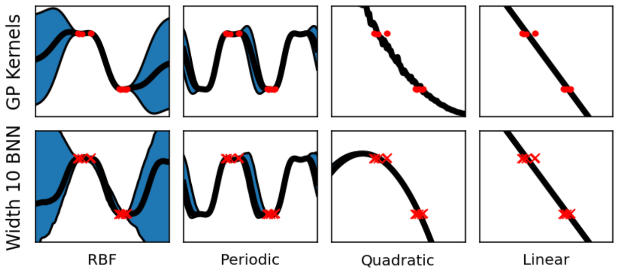
How might one translate a GP with compositional kernels into a BNN then? A single layer neural network will typically converge to a GP as the number of neurons (or "width") goes to infinity. More recently, researchers have discovered a correspondence in the other direction — many popular GP kernels (such as Matern, ExponentiatedQuadratic, Polynomial or Periodic) can be obtained as infinite-width BNNs with appropriately chosen activation functions and weight distributions. Furthermore, these BNNs remain close to the corresponding GP even when the width is very much less than infinite. For example, the figures below show the difference in the covariance between pairs of observations, and regression results of the true GPs and their corresponding width-10 neural network versions.

Comparison of Gram matrices between true GP kernels (top row) and their width 10 neural network approximations (bottom row).

Comparison of regression results between true GP kernels (top row) and their width 10 neural network approximations (bottom row).
Finally, the translation is completed with BNN analogues of the Addition and Multiplication operators over GPs, and input warping to produce periodic kernels. BNN addition is straightforwardly given by adding the outputs of the component BNNs. BNN multiplication is achieved by multiplying the activations of the hidden layers of the BNNs and then applying a shared dense layer. We are therefore limited to only multiplying BNNs with the same hidden width.
Using AutoBNN
The AutoBNN package is available within Tensorflow Probability. It is implemented in JAX and uses the flax.linen neural network library. It implements all of the base kernels and operators discussed so far (Linear, Quadratic, Matern, ExponentiatedQuadratic, Periodic, Addition, Multiplication) plus one new kernel and three new operators:
- a
OneLayerkernel, a single hidden layer ReLU BNN, - a
ChangePointoperator that allows smoothly switching between two kernels, - a
LearnableChangePointoperator which is the same asChangePointexcept position and slope are given prior distributions and can be learnt from the data, and - a
WeightedSumoperator.
WeightedSum combines two or more BNNs with learnable mixing weights, where the learnable weights follow a Dirichlet prior. By default, a flat Dirichlet distribution with concentration 1.0 is used.
WeightedSums allow a "soft" version of structure discovery, i.e., training a linear combination of many possible models at once. In contrast to structure discovery with discrete structures, such as in AutoGP, this allows us to use standard gradient methods to learn structures, rather than using expensive discrete optimization. Instead of evaluating potential combinatorial structures in series, WeightedSum allows us to evaluate them in parallel.
To easily enable exploration, AutoBNN defines a number of model structures that contain either top-level or internal WeightedSums. The names of these models can be used as the first parameter in any of the estimator constructors, and include things like sum_of_stumps (the WeightedSum over all the base kernels) and sum_of_shallow (which adds all possible combinations of base kernels with all operators).

Illustration of the sum_of_stumps model. The bars in the top row show the amount by which each base kernel contributes, and the bottom row shows the function represented by the base kernel. The resulting weighted sum is shown on the right.
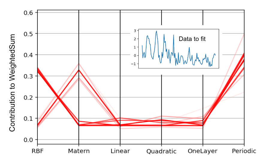
The figure below demonstrates the technique of structure discovery on the N374 (a time series of yearly financial data starting from 1949) from the M3 dataset. The six base structures were ExponentiatedQuadratic (which is the same as the Radial Basis Function kernel, or RBF for short), Matern, Linear, Quadratic, OneLayer and Periodic kernels. The figure shows the MAP estimates of their weights over an ensemble of 32 particles. All of the high likelihood particles gave a large weight to the Periodic component, low weights to Linear, Quadratic and OneLayer, and a large weight to either RBF or Matern.

Parallel coordinates plot of the MAP estimates of the base kernel weights over 32 particles. The sum_of_stumps model was trained on the N374 series from the M3 dataset (insert in blue). Darker lines correspond to particles with higher likelihoods.
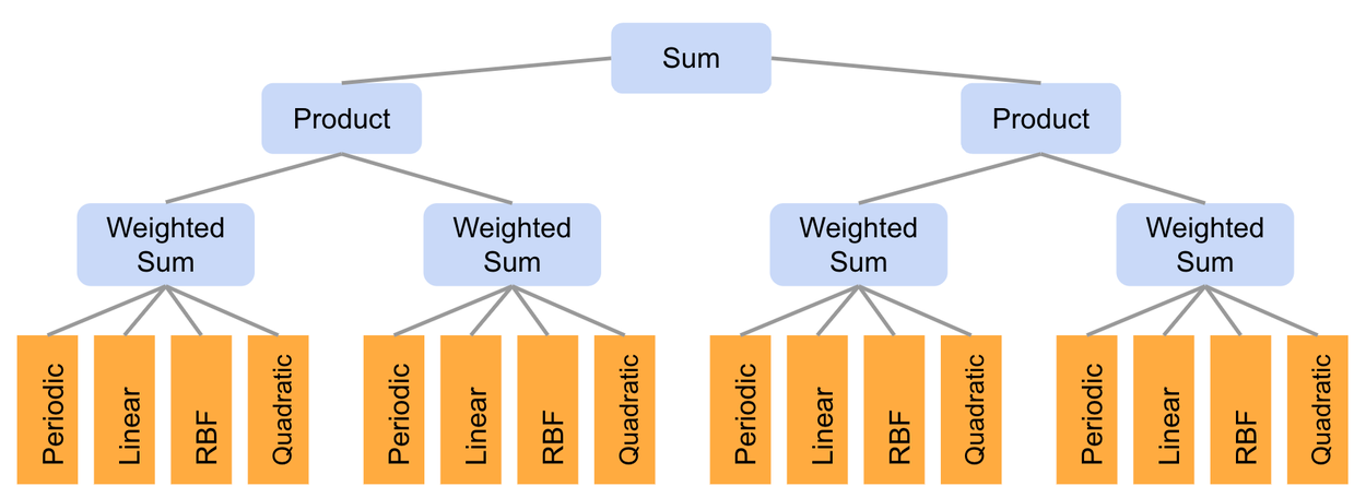
By using WeightedSums as the inputs to other operators, it is possible to express rich combinatorial structures, while keeping models compact and the number of learnable weights small. As an example, we include the sum_of_products model (illustrated in the figure below) which first creates a pairwise product of two WeightedSums, and then a sum of the two products. By setting some of the weights to zero, we can create many different discrete structures. The total number of possible structures in this model is 216, since there are 16 base kernels that can be turned on or off. All these structures are explored implicitly by training just this one model.

Illustration of the "sum_of_products" model. Each of the four WeightedSums have the same structure as the "sum_of_stumps" model.
We have found, however, that certain combinations of kernels (e.g., the product of Periodic and either the Matern or ExponentiatedQuadratic) lead to overfitting on many datasets. To prevent this, we have defined model classes like sum_of_safe_shallow that exclude such products when performing structure discovery with WeightedSums.
For training, AutoBNN provides AutoBnnMapEstimator and AutoBnnMCMCEstimator to perform MAP and MCMC inference, respectively. Either estimator can be combined with any of the six likelihood functions, including four based on normal distributions with different noise characteristics for continuous data and two based on the negative binomial distribution for count data.

Result from running AutoBNN on the Mauna Loa CO2 dataset in our example colab. The model captures the trend and seasonal component in the data. Extrapolating into the future, the mean prediction slightly underestimates the actual trend, while the 95% confidence interval gradually increases.
To fit a model like in the figure above, all it takes is the following 10 lines of code, using the scikit-learn–inspired estimator interface:
import autobnn as ab

model = ab.operators.Add(
    bnns=(ab.kernels.PeriodicBNN(width=50),
          ab.kernels.LinearBNN(width=50),
          ab.kernels.MaternBNN(width=50)))

estimator = ab.estimators.AutoBnnMapEstimator(
    model, 'normal_likelihood_logistic_noise', jax.random.PRNGKey(42),
    periods=[12])

estimator.fit(my_training_data_xs, my_training_data_ys)
low, mid, high = estimator.predict_quantiles(my_training_data_xs)
Conclusion
AutoBNN provides a powerful and flexible framework for building sophisticated time series prediction models. By combining the strengths of BNNs and GPs with compositional kernels, AutoBNN opens a world of possibilities for understanding and forecasting complex data. We invite the community to try the colab, and leverage this library to innovate and solve real-world challenges.
Acknowledgements
AutoBNN was written by Colin Carroll, Thomas Colthurst, Urs Köster and Srinivas Vasudevan. We would like to thank Kevin Murphy, Brian Patton and Feras Saad for their advice and feedback.


